(This is a huge project for me, since some details are even confusing for myself, I’m still a beginner of this field, this blog will be innovated inconstantly. It’s all up to my mood ^_^.)
This is an introductory article to a famous problem appeared in the Hamiltonian Dynamical Systems (and Symplectic topology), the Arnold conjecture, and a brief idea, which originated from Andreas Floer, to prove this conjecture. Let’s first start from the Morse theory.
1 Morse Homology
1.1 General Idea of Marston Morse
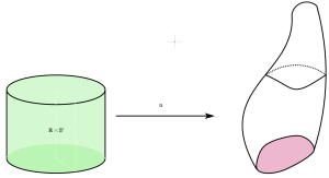
From a nowadays perspective of the geometry (probably due to Grothendieck and Serre), studying the geometry of a space 


Morse theory is a prior example of this philosophy. Morse’ idea was wishing to use a “Nice” function 

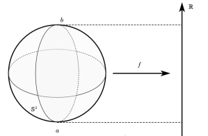
 , with 2 critical points on the south and north pole
  .
.It is proved that Morse functions are vastly existed on every compact manifold, hence it is a great tool that can help with the investigation of the topology of that manifold, a well-known application is that a critical point of a Morse function corresponds to a cellular structure of the underlying manifold.
Near each critical point 


The negative index 


There is also another (more intuitively) way to find the index of a critical point.
If we impose a Riemannian structure 


the field 


And the critical points of the Morse function

They are called the stable and unstable (sub)manifold of the critical point 

Theorem 1.1: 

More precisely, the unstable submanifold 

As another example, the following figure shows the critical points of the height function on a torus 


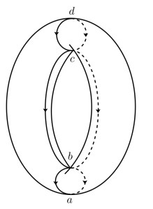
Also, it is not hard to find the gradient flow line flows from high index critical point to the low index one.
1.2 Morse Complex
Although, we know from the homological axiom that all homologies must be equal, but it is still necessary to construct homology functor from different aspects, for they offer us various ways in the comprehension of the object, the simplicial homology came through the simplicial decomposition, the de Rham cohomology came through the analysis on manifold, however, the Morse homology is constructed through a view from dynamical system.
We define the 

That is a free 

In order to define the boundary map, we need to find the connection between the critical points in successive indices, however, we need to impose an extra hypothesis.
We call a gradient field 


We denote by 

The Lie group 


So now, if two critical points are of successive indices, then 


It is pretty not easy to show that:
Theorem 1.2: The following is a chain complex:

Hence it determines a homology group in 
This homology group is called the Morse homology. Notice that, if we impose an orientation on 

It can be proved that the Morse homology has functoriality, hence it has all properties of other homologies, for example, Künneth formula, Poincaré duality, homotopy invariance, etc. Moreover, it is no wonder that the Morse homology coincide with the cellular homology, i.e., there is a natural isomorphism between these two chain complexes.
What a surprising result of the Morse homology is that it can help to evaluate the number of the critical points of a Morse function.
Theorem 1.3 (Morse Inequality): The number of critical points of a Morse function

Proof: It is obviously that:

Now, it is appropriate to end the story of Morse theory, right now.
2 Hamiltonian Dynamics
2.1 Hamiltonian Equations
Now we assume our 


for all 

The relationship between Hamiltonian vector field and the gradient vector field is subtle. Recall that there is a compatible almost complex structure 


and 


So, the Hamiltonian field is just a “twisted” gradient field.
The flow of a Hamiltonian is given by the ode:

If we write down in a local Darboux chart 


and assume 

The flow 


As a simple example, one can consider the height function 

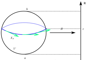 are the wefts
 Like the case in the gradient flow (it preserves the Riemannian structure), the Hamiltonian flow preserves the symplectic structure, that is 

2.2 Periodic Solutions
There is a significant concept in Hamiltonian dynamical systems, that is the periodic orbits/solutions of a Hamiltonian system. An orbit (or I shall say, the Hamiltonian flow line) of the Hamiltonian flow 


It is obviously that the critical points of 

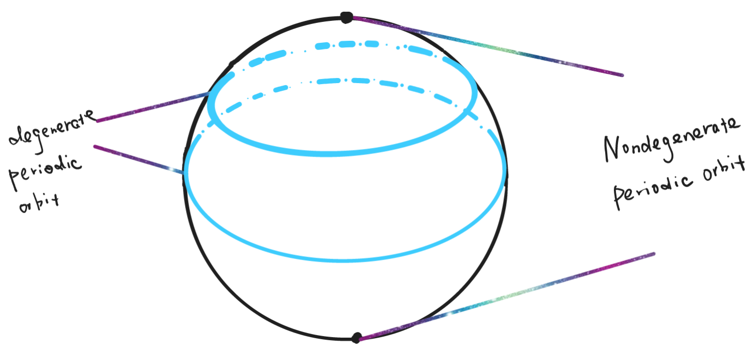
As an analogue in Morse theory, we can also define what is a nondegenerate periodic orbit.
Definition 2.1: A periodic orbit (of periodic 1) 
Intuitively, the nondegeneracy of a periodic orbit requires the orbit cannot be “too large”, for if so, we have the subspace 

The relation between nondegenerate periodic orbits and nondegenerate critical points is a little subtle:
Theorem 2.1: If a critical point of 

Proof: For the first statement, by definition, we have for all
![\begin{aligned}(d^2H)_x(u,v)&=(d(dH)_x)_uv=-(d\iota_{X_H}\omega_x)_uv\\&=-\left(\mathcal{L}_{X_H}\omega\right)_x(u,v)\qquad\text{(Cartan magic formula)}\\&=\omega_x([X_H, \tilde{v}]_x,u)\end{aligned}](https://s0.wp.com/latex.php?latex=%5Cbegin%7Baligned%7D%28d%5E2H%29_x%28u%2Cv%29%26%3D%28d%28dH%29_x%29_uv%3D-%28d%5Ciota_%7BX_H%7D%5Comega_x%29_uv%5C%5C%26%3D-%5Cleft%28%5Cmathcal%7BL%7D_%7BX_H%7D%5Comega%5Cright%29_x%28u%2Cv%29%5Cqquad%5Ctext%7B%28Cartan+magic+formula%29%7D%5C%5C%26%3D%5Comega_x%28%5BX_H%2C+%5Ctilde%7Bv%7D%5D_x%2Cu%29%5Cend%7Baligned%7D&bg=ffffff&fg=444444&s=0&c=20201002)
where 


![[X_H, \tilde{v}]_x\neq 0](https://s0.wp.com/latex.php?latex=%5BX_H%2C+%5Ctilde%7Bv%7D%5D_x%5Cneq+0&bg=ffffff&fg=444444&s=0&c=20201002)

Indeed, we choose 


![(d\phi^t_H)_x[X_H,\tilde{v}]_x\neq 0](https://s0.wp.com/latex.php?latex=%28d%5Cphi%5Et_H%29_x%5BX_H%2C%5Ctilde%7Bv%7D%5D_x%5Cneq+0&bg=ffffff&fg=444444&s=0&c=20201002)
For the second statement, if we use the local coordinates, the matrix of

where 


The existence of periodic orbits is a core and hard question in Hamiltonian dynamical systems, there is a big conjecture associate to this question, which conjectures the lower bound of the number of nondegenerate periodic orbits of a certain Hamiltonian system, that is the Arnold conjecture.
3 From Morse to Arnold
One of the reasons why I want to write this blog is that I want to make us sure why Arnold conjectured so, instead of conjecturing something others. If we know why it may true, this will give us an appropriate motivation to learn the forthcoming materials, such as Floer homology, Maslov index, Fredholm theory, etc.
Combining with section 2.2 and Morse inequality (theorem 1.3), we have the following simple corollary:
Theorem 3.1: We assume all periodic-1 orbits of a Hamiltonian 
Here, our Hamiltonian dynamical system is an autonomous system, which means 

V.I.Arnold conjectured the following:
Conjecture 3.2 (Hamiltonian Arnold Conjecture): We assume all periodic-1 orbits of a nonautonomous Hamiltonian 

There is also another more topological version of Arnold conjecture, called the Lagrangian intersection Arnold conjecture:
Conjecture 3.3 (Lagrangian Intersection Arnold Conjecture): Suppose 


The conjecture 3.3 implies the conjecture 3.2, however, the Lagrangian intersection one will not be considered in this blog.
Just one more remark about Arnold conjecture 3.2, that is the Hamiltonian 
Theorem 3.4 For any non-autonomous Hamiltonian systems 


Proof Let 
![[0,1]](https://s0.wp.com/latex.php?latex=%5B0%2C1%5D&bg=ffffff&fg=444444&s=0&c=20201002)


It is obviously that 


Many mathematicians made their efforts to solve these conjures, it was Andreas Floer who developed a method, called the Floer homology, which is an analogue of the Morse theory in infinite dimensional, and proved both conjectures, the later one is so called the Lagrangian intersection Floer homology. Meanwhile, there are a lot of “particular” version of the Arnold conjecture which can be proved via different theories, for example, Tamarkin and some other mathematicians used the “micro-local sheaf theory” proved the Lagrangian intersection Arnold conjecture for the cotangent bundle 
Next, we will talk about the Floer homology originated from the Hamiltonian dynamical case.
4. An Approach of Andreas Floer
Since we are focusing on the “loops” inside a symplectic manifold

This space endows with a 

Floer’s idea was to do the Morse theory on this loop space 

4.1 Loop Space & Action Functional
For loop space
For any loop 


with 


Convention 4.1: (1). For a curve on 
(2). For a tangent vector in
Another important notion is about the action functional, which will play an analogy role in Floer homology as Morse functions play in the Morse homology. Let

to be the action functional on the loop space 


Obviously, it is not well-defined since the action functional varies as the extension varies, but if we impose an extra condition 

where 

Next, I will compute the tangent map of this action functional.
Theorem 4.1: We have the tangent map 

Proof. To compute the tangent map, we choose a path 


Now, by definition we have:

For first term, by chain rules we have

For second term, by applying Cartan’s magic formula, we have

Combining with all these results, we gain the desired formula, cool!
Now, it is not hard to find the relationship between nondegenerate periodic-1 orbits and critical points of the action functional 
Theorem 4.2 A loop 
So now, we shall be awarded of what we need to play Morse theory on this action functional, here is the table of “menu”:
| Morse Theory | Floer Theory |
| Finite dimensional Manifold | Banach manifold |
Morse function  | Action functional  |
| Critical points of | Critical “loops” of |
| Morse index of critical points | Maslov index of critical “loops” |
| Equation of gradient flow | Floer equation |
| Counting flow lines connecting two critical points with successive index | Counting the number of solutions to Floer equation |
| Morse homology | Floer homology |
Next, I will introduce those analogously notions in Floer theory
4.2 Flow Lines Connecting Two Critical Points
Since for now, the periodic orbits are all critical points of the action functional, just as what we have done in Morse homology, we need to investigate the flow lines connecting them, we first start from the gradient of the action functional.
There is an 

for all 


Now it allows us to define the gradient vector field 

Combining with theorem 4.1, we have
Theorem 4.3: We have

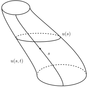
Now we can compute the flow line of the minus gradient field, let 

This equation is called Floer equation, notice that Floer equation is very similar to Cauchy-Riemann equation, since the first 2 terms is just Cauchy-Riemann equation, with a gradient of
Recall that we only care about those smooth contractible and periodic-1 solutions in 
……
Next, we will introduce the index of these critical “loops”, they are materials to make Floer chain groups, and how to count the number of the solutions of Floer equation, they are materials to make Floer boundary map.
5 Reference
- Michèle Audin, Morse Theory and Floer Homology, Springer-Verlag.
- V.I. Arnold, On a Topological Property of Globally Canonical Maps in Classical Mechanics, 1965
- C. Viterbo, An Introduction to Symplectic Topology Through Sheaf Theory
