On the Characteristic Varieties on Surfaces

Dedicated to Lin-Fang Hou, Wen Shen, Zheng-Tong Xie, Jing-Hong Deng, Hong-Jie Chow, Sang-Hao Xing and Jia Fei
In a memory to the fear during the past times provided by the reading seminar on M. Audin’s book.

The $G-$ characteristic variety $\mathcal{M}_{G}(M)$ of a manifold $M$ is the moduli space of representations of the fundamental group $\pi_1(M)$ into $G$ , from Riemann-Hilber correspondence, we know it parametrized the moduli space of flat connections on $M$ . The moduli space $\mathcal{M}_G(M)$ contains very important topological information of $M$ , and it plays a significant role in gauge theory, algebraic geometry and low-dimensional topology. This blog will give some simple examples of characeristic varieties on Riemann surfaces

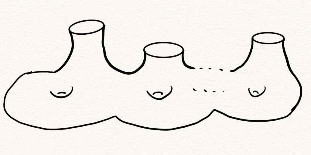
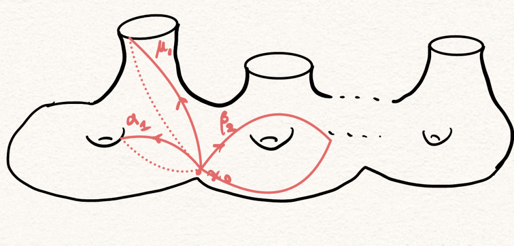
Let $\Sigma_{g,d}$ be a Riemann surface with genus $g$ and $d$ boundaries. Topologically, it looks likes the following:

Let’s pick a compact Lie group $G$ , the Riemann-Hilbert correspondence told us the following:

Theorem (Riemann-Hilbert): The space of pairs $(P,A)$ , where $P$ is a principal $G-$ bundle over $\Sigma_{g,d}$ and $A$ is a flat connection, modulo the gauge equivalence is isomorphic to the $G-$ characteristic variety of $\Sigma_{g,d}$ :

$\begin{aligned}\mathcal{M}_{g,d}^G=\frac{\mathrm{Hom}(\pi_1(\Sigma_{g,d});G)}{\mathrm{Ad}G}\end{aligned}$

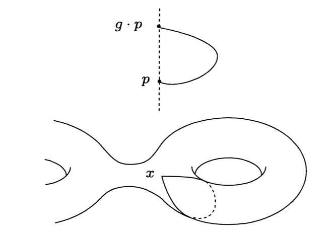
Sketch of the proof. For a flat connection $(P,A)$ , the holonomy defined by $A$ (a $\mathfrak{g}-$ valued 1-form on $P$ ) is a representation:

$\mathrm{Hol}_A: \pi_1(\Sigma_{g,d},x_0)\longrightarrow G$

for a loop $\gamma\in\pi_1(\Sigma_{g,d})$ based at $x_0\in \Sigma_{g,d}$ , the holonomy $\mathrm{Hol}_A(\gamma)$ is defined as follows: consider a horizental lift of $\gamma$ to $\tilde{\gamma}: [0,1]\longrightarrow P$ , where $\tilde{\gamma}(0)=(x_0,1_G)$ , at other points it satisfies an ODE:

$\begin{aligned}A_{\tilde{\gamma}(t)}\left(\frac{d\tilde{\gamma}(t)}{dt}\right)=0\end{aligned}$

the holonomy $\mathrm{Hol}_A(\gamma)$ is simply the fiber of $\tilde{\gamma(1)}$ .

To construct the reverse side, let’s consider the universal cover $\tilde{\Sigma}_{g,d}$ of $\Sigma_{g,d}$ , then every representation $\rho: \pi_1(\Sigma_{g,d},x_0)\longrightarrow G$ defines a principal $G$ -bundle:

$\begin{aligned}P:=\tilde{\Sigma}_{g,d}\times_{\pi_1(\Sigma_{g,d},x_0)} G\end{aligned}$

where the fundamental group $\pi_1(\Sigma_{g,d},x_0)$ acts by Deck transformation on the universal cover and acts by $\rho$ on $G$ . Consider a trivial connection $A_0$ defined on the trivial bundle $\tilde{\Sigma}_{g,d}\times G$ , it is a pull-back (injection!) of a connection $A$ on $P$ , one can check that this $A$ is flat with holonomy provided by $\rho$ . $\blacksquare$

Recall that, the fundamental groups of Riemann surfaces have presentations in words. Let $\mu_1,...,\mu_d$ be the oriented loops which touch the boundaries, $\alpha_1,...,\alpha_g$ and $\beta_1,...,\beta_g$ be the meridians and wefts based at $x_0$ , then we have

$\begin{aligned}\pi_1(\Sigma_{g,d},x_0)=\left\langle\mu_1,...,\mu_d,\alpha_1,...,\alpha_g,\beta_1,...,\beta_g\left|\prod_{i=1}^d\mu_i\prod_{j=1}^g[\alpha_j,\beta_j]=1\right\rangle\right.\end{aligned}$

where $[\alpha_j,\beta_j]=\alpha_j\beta_j\alpha_j^{-1}\beta_j^{-1}$ is the commutator.

Therefore, the space of representations will be

$\begin{aligned}\mathrm{Hom}(\pi_1(\Sigma_{g,d});G)=\left\langle M_1,...,M_d,A_1,...,A_g,B_1,...,B_g\left|\prod_{i=1}^dM_i\prod_{j=1}^g[A_j,B_j]=1\right\rangle\right.\end{aligned}$

It is subspace of $G^{2g+d}$ . Recall the fact that every compact Lie group is an affine smooth real algebraic variety (Hilbert’s 5th problem), therefore, the space $\mathrm{Hom}(\pi_1(\Sigma_{g,d});G)$ is hypersurface, in general, it is a singular real algebraic variety, and after the quotient of the adjoint action of $G$ , the characteristic variety $\mathcal{M}_{g,d}^G$ is a singular quotient variety.

However, if we are lucky that $\mathrm{Hom}(\pi_1(\Sigma_{g,d});G)$ is smooth, the characteristic variety $\mathcal{M}_{g,d}^G$ will still have singularities, where the singularities are provided by the non-free point of the adjoint $G-$ action.

Notice that, a representation $\rho$ is non-free if and only if there exits a non-trivial $g\in G$ such that $g\rho(\gamma)=\rho(\gamma)g$ , hence $\rho$ is not an irreducible representation. Which is to say, the possible singularities are provided by the reducible representations. Moreover, at each regular point, the dimension of $\mathcal{M}_{g,d}^G$ can be computed by the dimension of the tangent space, it is:

$\dim \mathcal{M}_{g,d}^G=(2g+d-2)\dim G$

Here are 2 simple examples:

Example 1: Let $G=S^1$ which is an Abelian Lie group, thus the adjoint action is just trivial, and the characteristic variety $\mathcal{M}_{g,d}^{S^1}$ is just $\mathrm{Hom}(\pi_1(\Sigma_{g,d});S^1)$ . It is:

$\begin{aligned}\left\langle M_1,...,M_d,A_1,...,A_g,B_1,...,B_g\left|\prod_{i=1}^dM_i=1\right\rangle\right.\end{aligned}$

which is isomorphic to the torus $(S^1)^{2g}$ for $d=0$ , and $(S^1)^{2g+d-1}$ when $d\geq 1$ . $\blacksquare$

Example 2: Let’s consider a 3-holed sphere $\Sigma_{0,3}$ , and let $G=SU(2)$ . We have

$\mathrm{Hom}(\pi_1(\Sigma_{0,3});SU(2))=\langle M_1,M_2,M_3\in (SU(2))^3|M_1M_2M_3=I\rangle$

Recall that a matrix $SU(2)$ is adjoint to a diagonal one $\begin{pmatrix}e^{i\theta}& \\ & e^{-i\theta}\\ \end{pmatrix}$ . So, under the adjoint action, we can write $M_1=\begin{pmatrix}e^{i\theta_1}& \\ & e^{-i\theta_1}\\ \end{pmatrix}$ , where $\theta_1\in[0,\pi]$ .

Now, to preserve the diagonality of $M_1$ , we can keep using a diagonal elemnt to act on $M_2$ . Under this setting, $M_2$ will have a simple form $\begin{pmatrix}a& b\\ -b& \bar{a}\end{pmatrix}$ , where $b\in\Bbb{R}^+$ is real positive. Or more techniquely, we can assume $b=\sin \beta$ for some $\beta\in [0,\pi]$ , and $a=\cos\theta_2-i\sin\theta_2\cos\beta$ for some $\theta_2\in[0,\pi]$ .

Finally, since $M_1M_2M_3=I$ , we can determine the eigenvalues (adjoint type) of $M_3$ , we can assume

$\begin{aligned}M_1M_2=\begin{pmatrix}e^{i\theta_3}& \\ & e^{-i\theta_3}\\ \end{pmatrix}\end{aligned}$

Then $\theta_3,\theta_2,\theta_1$ and $\beta$ should satisfiy the relation

$\cos\theta_1+\sin\theta_1\sin\theta_2\cos\beta=\cos\theta_3$

Thus the moduli space $\mathcal{M}_{0,3}^{SU(2)}$ can be parametrized by those $\theta_i,\beta$ which satisfies the above trignometric equation.

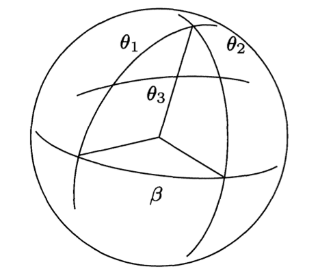
Recall that in shperical geometry, the above equation is the Cosine Formula of a spherical triangle, where $\theta_1,\theta_2,\theta_3$ are the length of edges of a spherical triangle, and $\beta$ is the angle determined by $\theta_1,\theta_2$ :

So, the characteristic variety $\mathcal{M}_{0,3}^{SU(2)}$ can be understood as the isometry classes of spherical triangles on a unit sphere $S^2$ , the singularities are where the triangle degenerates. On the other hand, we can send

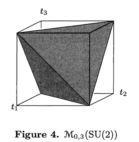
$\mathcal{M}_{0,3}^{SU(2)}\longrightarrow \Bbb{R}^3$ , $\begin{aligned}(\theta_i,\beta)\mapsto\frac{1}{\pi}(\theta_1,\theta_2,\theta_3):=(x_1,x_2,x_3)\end{aligned}$

By triangle axioms, we have $\mathcal{M}_{0,3}^{SU(2)}$ is isomorphic to the following tetrahedron:

$\begin{aligned}\left\{(x_1,x_2,x_3)\left| |x_1-x_2|\leq x_3\leq x_1+x_2, 0\leq x_i\leq 1, \sum_{i=1}^3x_i\leq 2\right\}\right.\end{aligned}$

it looks likes the following:

Moreover, the singularities of $\mathcal{M}_{0,3}^{SU(2)}$ are precisely the vortices and edges of this tetrahydron, such a space is called a cornered manifold. $\blacksquare$

Example 3: In the case $d=0, g\geq 2$ , and $G=PSL(2,\Bbb{R})$ , the characteristic variety $\mathcal{M}_{g}^{PSL(2,\Bbb{R})}$ is very important in conformal geometry. The component containing discrete representations (i.e. the image is a discrete subgroup of $PSL(2,\Bbb{R})$ ) forms a connected component, it is the famous Teichmüller space of the Riemann surface. It is isomorphic to the Euclidean space $\Bbb{R}^{6g-6}$ . The Teichmüller space will tell the deformation of the hyperbolic structures on $\Sigma_{g}$ . If we replace $PSL(2,\Bbb{R})$ by some more general Lie group, such as $PSL(n,\Bbb{R})$ , there is also a special component in the characteristic variety $\mathcal{M}_{g}^{PSL(n,\Bbb{R})}$ , which is called the Hitchin component. It is referred to a high analogue of the Teichmüller theory, namely, the higher Teichmüller theory. $\blacksquare$

More interesting things will happen on the characteristic variety. If we assume $G$ is simply connected, for example $G=SU(n)$ , then every princple $G-$ bundle over $\Sigma_{g,d}$ is trivial. So we can fix a principal bundle $P=\Sigma_{g,d}\times G$ , and the characteristic variety is the affine space of flat connections on $P$ modulo the gauge equivalence: $\mathcal{M}_{fl}=\mathcal{A}_{fl}(P)/\mathcal{G}$ , where $\mathcal{G}$ is the bundle transformation of $P$ , in this case, it is $C^{\infty}(\Sigma_{g,d},G)$ .

In 1982, Atitah and Bott gave a symplectic description of the moduli space $\mathcal{M}_{fl}$ . We shall first consider the affine space of connections $\mathcal{A}(P)$ , its tangent space is just $\Omega^{1}(\Sigma_{g,d},\mathrm{ad}P)$ , the $\mathfrak{g}-$ valued 1-forms on $\Sigma_{g,d}$ . There is a natrual symplectic form $\omega$ on $\mathcal{A}(P)$ :

$\begin{aligned}\omega_A(\phi_1,\phi_2)=\int_{\Sigma_{g,d}}\mathrm{Tr}(\phi_1\wedge\phi_2)\end{aligned}$

the term in the integrand can be understood as the Killing form on the Lie algebra $\mathfrak{g}$ .

In the case when $d=0$ , i.e. the Riemann surface has no boundaries, then Atiyah-Bott showed that $\mathcal{G}$ acts in a Hamiltonian fashion on the symplectic affine space $\mathcal{A}(P)$ , and the the moment map $\mu: \mathcal{A}(P)\longrightarrow \mathrm{Lie}(\mathcal{G})^*\cong\Omega^2(\mathrm{ad}P)$ is simply the curvature: $A\mapsto F_{A}$ , thus the moduli space of flat connections $\mathcal{M}_{fl}$ is the symplectic reduction hence a symplectic manifold.

If the surface has boundaries, then the symplectic structure on $\mathcal{A}(P)$ cannot induce a symplectic structure on $\mathcal{M}_{fl}$ but a Poisson structure. The symplectic leaves are constructed by fixing holonomies along the boundaries. What’s more, in 1984, William Goldman construced an integrable system on the moduli space $\mathcal{M}_{g,d}^{G}$ which is now called the Goldman system.

However, the exciting things are far from over. In the case of compact Riemann surfaces, the characteristic variety $\mathcal{M}_{g}^G$ earned more investigation, especially for its relation to the gauge theorotical equations. In 1987, Nigel Hitchin introduced the notion of Higgs bundles $(E,\Phi)$ , which is the solution of the Hitchin’s equations. Hitchin proved the solutions of his equations are gauge equivalent to the stable holomorphic Higgs bundles, hence they can be related to the characteristic variety $\mathcal{M}_{g}^G$ . Hitchin also constructed an integrable system, which is the celebrated Hitchin’s system, it plays an important role in understanding some other typical integrable systems, and it also shed its light in geometric Langlands Program.

My Tiny Math Home

On the Characteristic Varieties on Surfaces

留下评论取消回复

分享到：

留下评论 取消回复

留下评论取消回复